Analysis of British EIHL Ice Hockey Shot Data
Introduction
The Elite Ice Hockey League (EIHL) is the professional Ice Hockey league in the UK comprising of teams from all 4 nations of the UK. During the curtailed 2019-20 season, the EIHL started to record more advanced stats during each game. Previously, the only stats recorded were number of shots on target, number of penalty minutes accrued, who scored the goals and who provided the assists to each goal - each goal can have up to 2 assists: the player who passed the puck to the goalscorer (primary assist) and the player who passed the puck to the primary assist (secondary assist).
The new stats recorded were the players who were on the ice at the time of each goal and also a map of all shot attempts. I’ll be taking a look at the shot data, performing some exploratory data analysis exploring where teams take shots from, what positions goals are scored from, and where rebounds are generated - rebounds are often more difficult for goaltenders to save as they tend to be out of position after saving the initial shot. I’ll also build a shot quality model. The EIHL website only presents the raw shot map for each game, as well as some basic statistics about the where shots are taken, however this is only performed at the individual game level.
There are 2 concerns I had about the shot data before working with it:
- My understanding is that the data is recorded by someone sat in the stands with a tablet - this could lead to errors in the data and I am not sure whether video footage is used to correct this data after a game is complete (my assumption is that it is not used). It’s tough job trying to manually count shots as they happen as Ice Hockey is a fast-paced sport.
- Different arenas have different sized ice rinks. The size of the ice surface in Manchester is notoriously small (57 m x 26 m), while others are much larger (60 m x 30 m). This may not seem like much, however it does have an effect on the games and it may mean that the shot distribution is different in each arena. Olympic standard rinks are 60 m x 30 m, while rinks used in the NHL (USA & Canada) are 200 ft x 85 ft (61 x 26 m). After consulting The Hockey Forum it appears that Coventry (58 m x 26 m) & Fife (195 ft x 95 ft), as well as the aforementioned Manchester, have different sized rinks to the rest of the teams which all have Olympic sized ice.
Getting the Data
The individual shot maps are shown on the EIHL website - an example of which can be found here and is shown in the below screenshot

I’ll explain more about the data format shortly, however I first wanted to highlight how I scraped the data. The raw data is not contained on the EIHL website, rather the maps are hosted on a Czech website and embedded in the EIHL website. You can view the Cardiff shot map from above game here. This website only shows the visualisation of the map, it does not host the raw data. Inspecting the HTML of the shot map visualisation lead me to find that the raw data is stored in JSON files on an Amazon AWS server, the data for the example game can be found here.
Each game on the EIHL website has an integer match ID, the Cardiff-Dundee game above has ID 925. The raw data also contains a match ID, unfortunately this does not always match the ID on the EIHL website (I’m not sure why!). This meant to get all of the match IDs for the shot maps, I had to navigate to each match page in turn, find the corresponding ID, and grab the raw data. If the IDs had matched I would only have to navigate to the EIHL website once. To get the data I used the requests package in Python and I included a 10 second pause after scraping the data for each match to ensure that I did not make too many calls to any websites in a short time period.
The first step was to get the EIHL match IDs from the fixture list
fixtures_url = "https://www.eliteleague.co.uk/schedule?id_season=2&id_team=0&id_month=999"
fixtures_http = requests.get(fixtures_url)
idxs = [m.start() for m in re.finditer("a href=\"/game/", fixtures_http.text)]
Then I iterated through the EIHL match IDs, navigated to each match page and found the match ID from the shot map. Some of the code has been given below to illustrate this, although some steps have been removed for brevity.
track_url = "https://www.eliteleague.co.uk" +g_id + "/tracking"
track_html = requests.get(track_url)
ind2 = track_http.text.find("https://eihl.hokejovyzapis.cz/visualization/")
ind3 = track_http.text.find("\"",ind2)
s_id = track_http.text[(ind3-4):ind3]
if(s_id[0] == "="):
    s_id = s_id[1:]
if s_id not in game_ids:
    game_ids.append(int(s_id))
    json_url = "https://s3-eu-west-1.amazonaws.com/eihl.hokejovyzapis.cz/visualization/shots/" + str(s_id) + ".json"
    shots = requests.get(json_url).text
time.sleep(10)
The variable g_id is the EIHL match ID, and the variable s_id is the match ID from the shot map. The data from each shot map is retrieved from the JSON file as a dictionary, joined with together with the other matches, and a Pandas DataFrame was generated to store the values.
Data Format
The raw data contained a number of fields:
- ID, Player ID, Team ID, Opposition ID, Match ID - unique IDs for each shot, player, team (that the player plays for), opposition team, and match.
- Jersey Number
- Player First & Last Name
- Shot Result - 1 if the shot was saved, 2 if the shot was wide, 3 if the shot was blocked (not by the netminder), or 4 if the shot went in.
- Time - the time, in seconds, when the shot was taken.
- Coordinates - the coordinates where the shot was taken. Both $x$ & $y$ values range from $-100$ to $100$, with $(0,0)$ relating to the centre of the ice rink.
- Date & Time - the date & time of the shot.
- Home Game - whether the team was playing at home or away.
- Team & Opposition Team Names - the names of the teams playing the match.
To perform the analysis I added new fields to the DataFrame to include some extra information. The coordinates of the shots for the away team needed to be rotated by $180^{o}$ around the origin, I also calculated the distance that each shot was taken from and the time to the previous shot and time to the next shot - the latter values were used to calculate whether a shot resulted in a rebound or originated from a rebound.
Extra Data
The information provided in the shot data was insufficient to perform any analysis. It did not contain any information about how many players were on the ice or whether any of the shots were penalty shots - the probability of shots going in is most likely different depending on how many players on are the ice . To get this information I scraped the gamesheets from the EIHL website and extracted the goal and penalty information. This allowed me to ascertain whether each goal was a penalty shot or a delayed penalty goal, and the number of players on the ice when each shot was taken. I put the goal information in one DataFrame and the penalty information in another DataFrame.
Combining the DataFrames caused some problems - firstly there were 9 shots that were listed as goals in the shot data but were not actually goals. Rather than attempting to correct these I dropped them from the shots DataFrame. Secondly there were 5 shots that needed to be changed to goals in the shots DataFrame. The times of the goals in the gamesheet did not always match up with the times of the goals in the shot DataFrame. In fact in two cases it looks like some of the shots were listed as the wrong period - it was not possible to fix this as I did not know which shots were in the correct period and which were in the incorrect period in the DataFrame. Finally, some of the shots that were listed as goals were taken by players who were not listed as the goalscorer in the gamesheet. I was unsure whether these were due to deflected goals or mistakes by whoever inputted the data (it looks like a difficult job!) so I decided not to correct these. I did notice that a number of these goals appeared to the have the shooter (the player listed as taking the shot in the DataFrame) as the player with the assist in the gamesheets which could suggest the goal was a deflection.
The final piece of the puzzle was finding which goals were empty net goals - towards the end of the match when a team is down by 1 or 2 goals then they may switch their netminder with a skater for an increase change of a goal. Unfortunately, the data on this is not great - the gamesheet doesn’t contain a list of times when the netminder is out of the net, neither does the shot data. To get this data I had to go to the game webpage and scrape the information from the list of events (goals and penalties in order of time), then I had to match the time of the empty net goal(s) with the time of the goals which had previously been matched with the goals in the shots DataFrame.
Shot Statistics - Shot Attempts
Before generating heat maps I performed some basic analysis on the shot data. First let’s take a look at distribution of the shot outcomes.
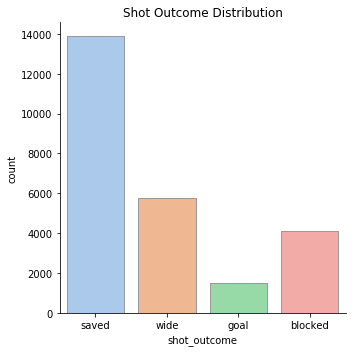
The good news, for the goalies at least, is that goals has the lowest counts! It’s also good to see that more shots are saved than go wide. 55% of all shot attempts were saved, 23% went wide, 16% were blocked, and the remaining 6% resulted in a goal. For all shots on target, 90.6% were saved - empty net goals have been accounted for in this value.
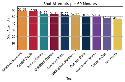
The number of shots per game for each team has been plotted below. It is clear that Sheffield and Cardiff sit above the other teams and they finished the season as the top 2 teams in terms of points per game (recall, the season finished early and not all teams played the same number of games). Fife are firmly at the bottom of this graph with the lowest number of shot attempts per game, they also had the lowest number of points per game and finished the season bottom of the table. Interestingly they did not score the fewest goals during the season, that was Manchester who took the 8th most shot attempts per game. We’ll dig further into the stats to see why this might be.
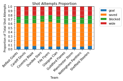
We can also look the proportion of shots that each team took that resulted in different outcomes. For example, Fife took the fewest shots but scored more than Manchester, so they had a better goals per shot attempt ratio. We can plot these ratios and I’ve also included them in the table below the plot which shows the number of each shot type per game.
| Team | Blocked | Goal | Saved | Wide |
|---|---|---|---|---|
| Belfast Giants | 7.77 (14.3%) | 3.06 (5.6%) | 30.34 (56.0%) | 13.02 (24.0%) |
| Cardiff Devils | 11.01 (19.0%) | 3.45 (6.0%) | 30.52 (52.6%) | 12.99 (22.4%) |
| Coventry Blaze | 8.94 (17.0%) | 3.69 (7.0%) | 28.57 (54.2%) | 11.54 (21.9%) |
| Dundee Stars | 7.02 (13.8%) | 2.98 (5.9%) | 29.50 (58.1%) | 11.28 (22.2%) |
| Fife Flyers | 6.90 (15.0%) | 2.51 (5.5%) | 27.01 (58.6%) | 9.65 (21.0%) |
| Glasgow Clan | 7.18 (15.0%) | 2.87 (6.0%) | 26.73 (55.4%) | 11.31 (23.5%) |
| Guildford Flames | 10.35 (19.5%) | 3.05 (5.7%) | 27.81 (52.3%) | 11.91 (22.4%) |
| Manchester Storm | 6.80 (13.5%) | 2.29 (4.5%) | 29.70 (58.7%) | 11.74 (23.2%) |
| Nottingham Panthers | 7.75 (14.8%) | 3.13 (6.0%) | 27.65 (53.0%) | 13.68 (26.2%) |
| Sheffield Steelers | 11.15 (18.9%) | 4.29 (7.3%) | 30.31 (51.5%) | 13.14 (22.3%) |
A few things stand out from this data. Firstly, almost 1 in 5 shot attempts by Guildford were blocked, followed by Cardiff and Sheffield. We will look at where these shots originate from later on in this article. We can also see that Nottingham are missing over 1 in 4 of their shot attempts, the highest in the league. Sheffield and Coventry are scoring the highest proportion of their shots with 7.3% and 7.0%, respectively. Manchester are the other extreme in this case, scoring only 4.5% of their shot attempts, while they had the highest proportion of saved shots (58.7%) suggesting that their players were getting the puck on net but struggling to score. Manchester would have to take 155 shot attempts to score the same number of goals as Sheffield would in 100 shot attempts.
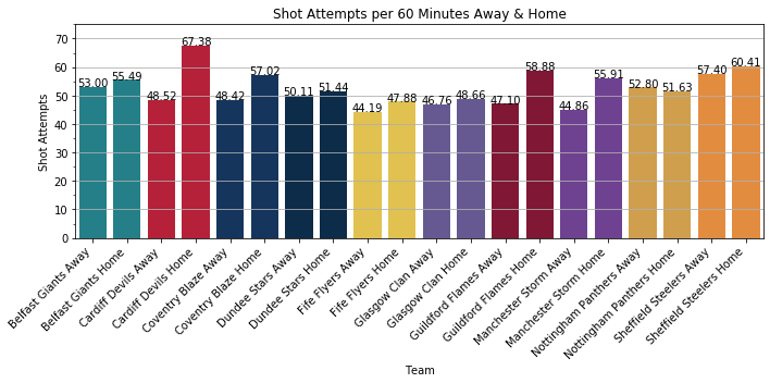
We can also look at splitting this data into home and away games, which is shown below. From this we can see some teams have a large difference in the number of shot attempts at home compared to when playing away. Cardiff shows the largest swing, followed by Guildford and Manchester. Nottingham were the only team who had more shot attempts per game away from home.
Let’s flip this and see how many shots per game teams are giving up each game. Below we see the number of shot attempts, and below that we see the data split up into home and away.
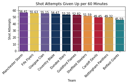
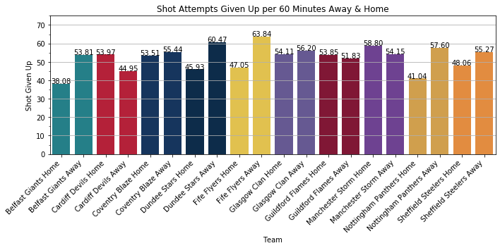
We can see that Manchester give up the most shot attempts per game, followed by Fife and Glasgow. Belfast were the ‘stingiest’ team, giving up more than 10 shots fewer per game than Manchester. We can also see that Cardiff, Manchester, and Guildford give up more shots at home than away. At Manchester this could be due to the smaller ice size, although I’m not sure why this is the case for Cardiff and Guildford. We can also see that Nottingham have the largest difference between Home & Away, giving up over 16 shot attempts per game more away from home. As Nottingham also took fewer shots home than away this could suggest that shots are being undercounted at their home arena (or shots are being overcounted in other arenas) or it might be due to tactics, it’s difficult to tell without extra data.
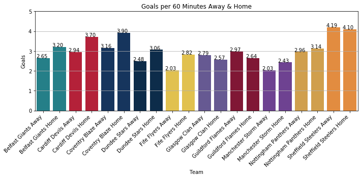
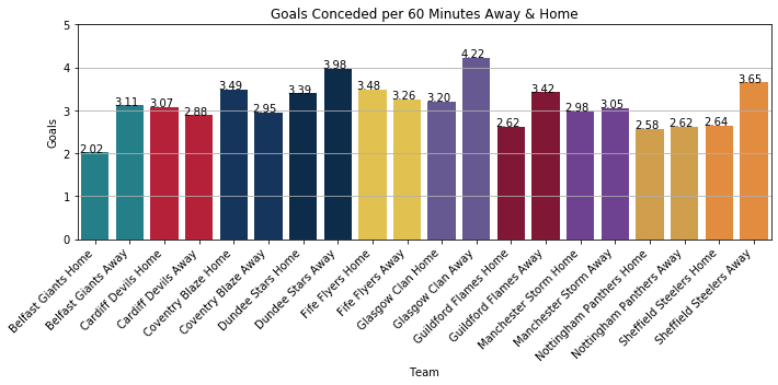
Finally, we’ll take a look at the goals per 60 minutes for each team, split home & away, as well as the number of goals conceded per 60 minutes for each team. I have removed empty net goals from these graphs as these are special cases. Interestingly 3 teams - Glasgow, Guildford, Sheffield - scored more goals per 60 minutes away than at home, while Cardiff, Coventry, and Fife conceded more goals per 60 minutes at home than away.
Team-by-team Shot Heat Maps
To generate the shot heats maps I used the matplotlib and seaborn libraries, in particular I used the kdeplot function in seaborn which plots a (in this case) bivariate kernel density estimate. I used the default values for the kernel (Gaussian) and the bandwidth (the Scott method). The Scott method uses n**(-1./(d+4)) to calculate the bandwidth, where $n$ is the number of data points and $d$ is the number of dimensions. The kernel density estimates were overlaid on top of the rink image used for the EIHL shot maps.
These first set of maps were generated from shots taken at home (to avoid any issues relating to the size of the rink) and include all types of shot attempt.
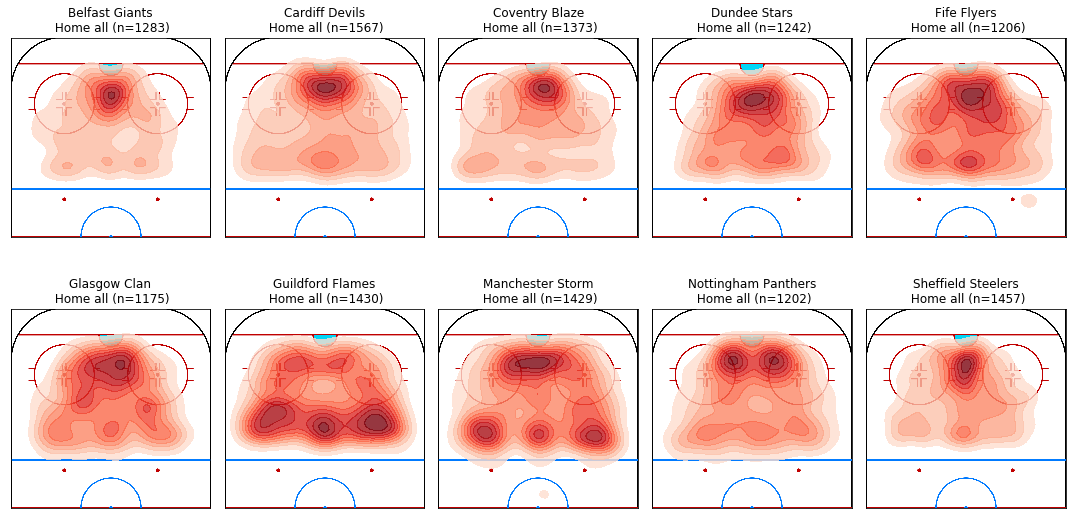
We can see that there is a region close to the goal where all teams tend to have a large number of shots from. For Nottingham and Guildford there appears to be two regions close to the goal, with a slightly lower chance of a shot attempt from right in front of the goal. We also see a number of shots being taken from near the blue line, with some teams having a larger proportion of shots from this region (for example Guildford and Manchester) compared to others. Upon looking at this my first thought was maybe teams who were lower down in the league table may have a larger proportion of shots from further away from goal as perhaps they don’t spend as much time as close to the goal, and this appears to be the case on first glance looking at Fife, Dundee, Manchester, Glasgow, and Guildford (the 10th - 6th placed teams). Guildford also have a couple of defencemen who are well known for shooting the puck, so this may explain why they tended to shoot from further away.
By taking the average across all of the teams shot maps, we can take the ratio between each teams map and the average to see whether certains teams tend to shoot from further away. These have been shown below, where red indicates a team has a higher than average proportion of shots from a region and blue indicates a team has a lower than average proportion of shots from a region. White indicates the team matches the average proportion of shots for that region.
The maps have been plotted on a logarithmic scale and the area behind the goal and near the half way line have been omitted due to the low number of shots taken from these regions. The maps show that Belfast, Cardiff, Coventry, Nottingham, and Sheffield all had a higher proportion of shots in the region directly next to the goal than the other teams. These teams also scored the highest number of goals per game, with the exception of Nottingham who scored 3.26 goals per home game which was 6th overall, 1 place behind Dundee with 3.27 goals per home game. Note that Dundee’s shots tended to be more central which may explain why their scoring was a bit higher. We can also see that Manchester had a higher proportion of shots from wider on the ice, this might be due to the smaller sized rink at Manchester.
Now that we’ve looked at where shots are taken from we’ll take a look at where goals are scored from. The heat maps for each team for home goals have been shown below.
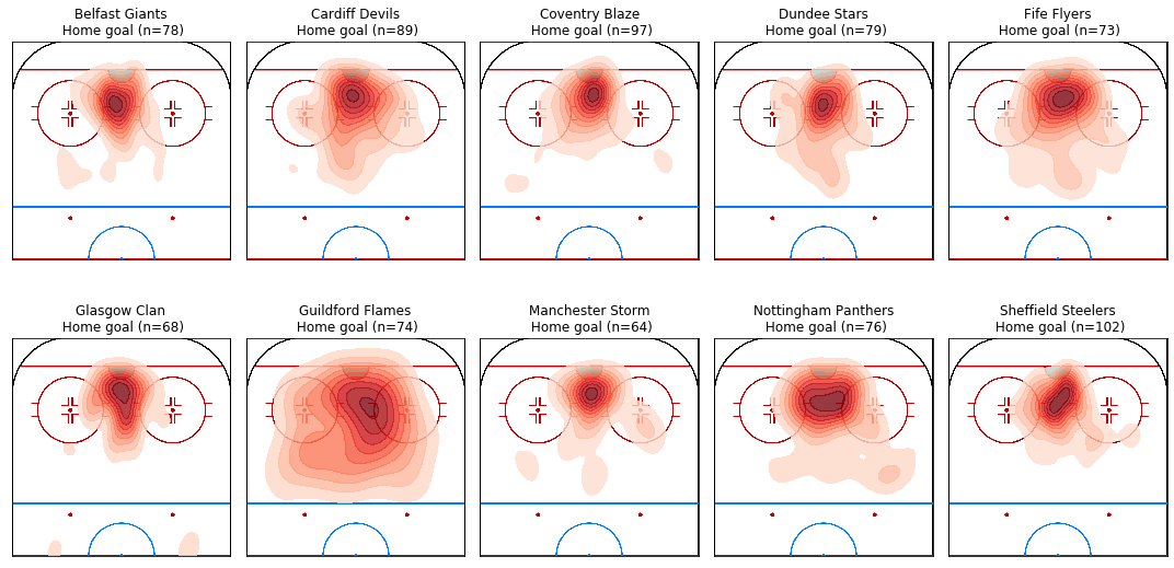
It’s clear from these maps that most goals are scored in the region between the goal crease and the two face off circles. The one noticeable outlier is Guildford who scored more goals from further away than other teams - this is not suprising as we previously saw that Guildford take more of their shots from further away as well.
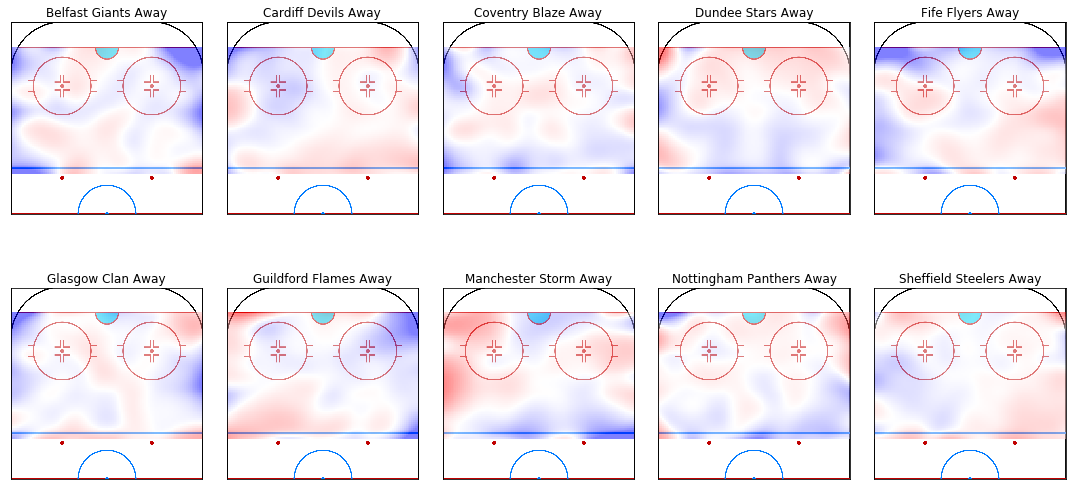
We’ll now take a look at the same heat maps, but for games played away from home. First, let’s take a look at where all shot attempts were taken from for each team away from home. Recall that Manchester, Coventry, and Fife have smaller rinks than the rest of the league and therefore averaging over away rinks like this may cause some problems.
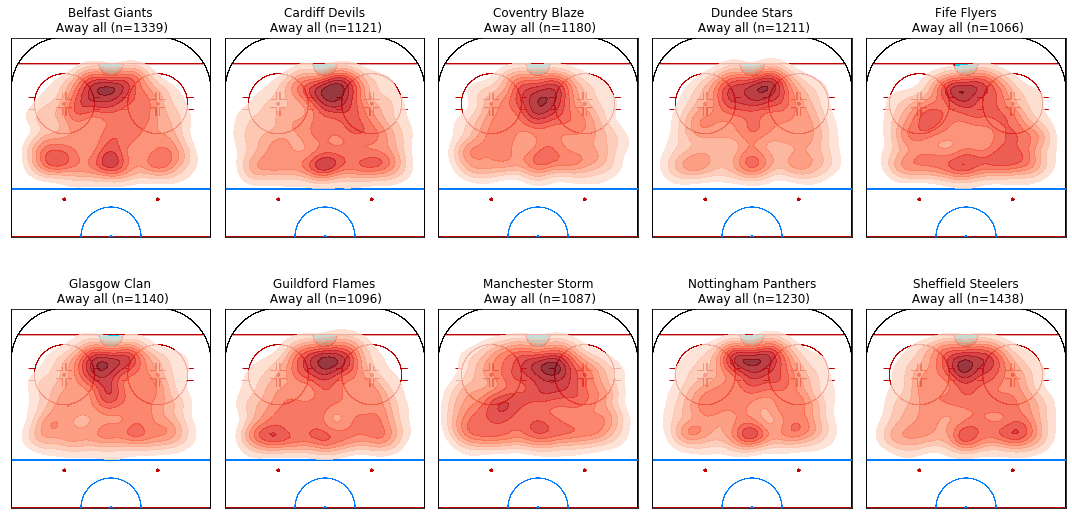
Performing a visual comparison by eye it appears that teams are taking more shots from further away from the goal. This would make sense as teams tend to play more defensively when they’re away from home, perhaps they’re restricted to shots further away from the goal?
We can also take the ratio between the heat maps and the average away team heat map, which have been visualised below. Again, a visual inspection suggests that there is much less team-to-team variation than when comparing home shots, the values in these maps vary much less from the average than previously.
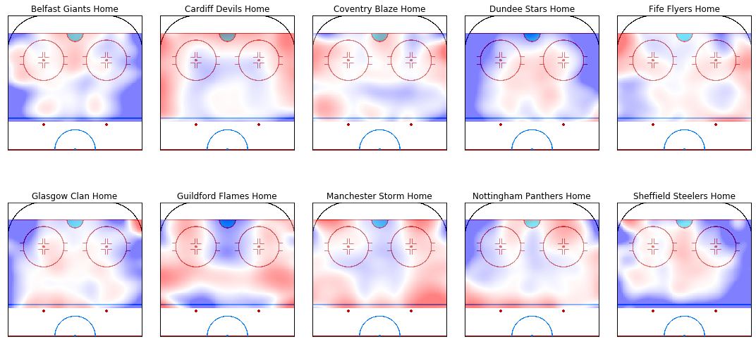
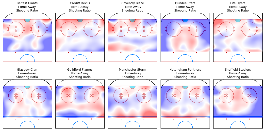
Rather than compare each team to the average, we can compare each team’s home shooting map with their away shooting map. This has been shown below, red meaning a team has a higher proportion of shots at home in a region than away. Note that this shows the tendency for shots to be taken from region, and the number of shots has been normalised (recall teams tend to have more shots home than away). It’s difficult to see any trends here, although in general the region close to the goal is red - i.e. teams take a higher proportion of shots closer to the net at home than away. The exceptions are Dundee, who took a lot of shots at home in the centre of the ice between the faceoff circles and further away, Guildford who take a lot of shots from the blueline as discussed earlier, and maybe Nottingham who took a higher proportion of central shots away but tended to shoot from off-centre at home.
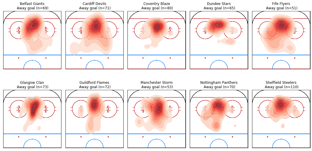
Finally, let’s look at the goal heat maps. It looks like teams are scoring a higher proportion of their goals from further away from the net than at home. The largest change appears to be Guildford who are scoring more goals from closer in than at home.
Shot & Goal Distance
The shot maps suggest that teams tend to shoot from further away from goal when playing away, and different teams have different shooting habits. They also suggest, in general, that goals tend to be scored from closer to the goal. We can explore these by histogramming the distance that shots are taken from and goals are scored from. First, let’s overlay a distance contour map on top of an Olympic sized ice rink, so we understand how far different regions are on the ice.
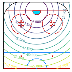
The goal heat maps shown previously suggest that most goals are scored from within 10 m or so, let’s take a look at histogramming the shot and goal distances.
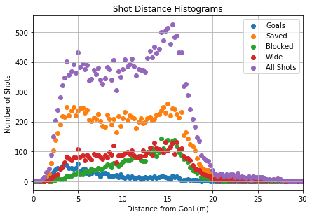
The above plot shows the distribution of the distances of the different kind of shots (excluding empty net goals), which have been histogrammed to the nearest 0.25 m. We can see that there is an initial peak at around 5 m before a plateau to approximately 12.5 m and then a peak at 15 m before a steep decline. 5 m is quite close to goal and we saw a large concentration of shots being taken from here in the shot heat maps. The shots from 15 m are coming from inside the blueline where defencemen tend to take shots, and the plateau in between could be off-centre shots (wingers taking shots) and more central but slightly away from the goal. Looking at saved shots we see that there are approximately the same number of saves from 5 m as there are at 15 m with a dip in between (perhaps there is a slight peak at 10 m as well). Blocked shots are clearly more likely to occur from 15 m than from close in, which makes sense as you’d expect there to be more players between the shooter and the goal when the shot is taken from further away. There is also a slightly higher number of wide shots from further away than close together, again this is expected as the goal is larger (in terms of solid angle) the closer to the goal. Finally, we can see that goals tend to be scored at 5 m or less, with the peak occuring 3.5 m from the goal.
From these plots we can estimate the probability that a shot from a particular distance will result in a goal, go wide, be saved, or be blocked. We need to be careful when calculating these as the low numbers of shots from close in and long-range may lead to shots from some distances having a 100% chance of being a goal.
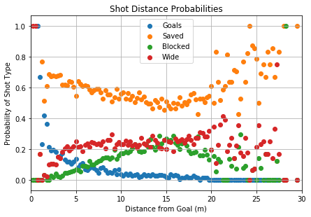
As we saw in the previous plot, the number of shots from closer than 2 m was very low, in fact there were only 100, which explains why the probability of scoring goals from close in is very high. Looking at goals there appears to be a very clear trend between the probability of a shot being a goal and distance, with a few outliers possibly caused by low statistics or data errors. The probability of a shot being blocked peaks at around 15 m, while the probability of a shot going wide appears to be relatively constant after 4 m or so at just over 20% until approximately 20 m from the net where again low statistics causes some issues. The probability of a shot being saved looks a bit parabolic, starting quite high (due to a lack of wide and blocked shots close in) before dropping down to approximately 50% at 15 m from the net before increasing again.
Powerplays & Rebounds
So far I’ve lumped most of the data together, however this covers a wide range of scenarios and shot types. Unfortunately the type of shot (slap, wrist, one timer, backhand) is not recorded, however, we can estimate whether a shot is rebound or not by looking at the time between shots. I will classify a rebound as a shot following a save only (not a shot that went wide or was blocked) that occured within a certain time period after the initial shot. Previous analysis of NHL shots considers a rebound if the shot was within 2 seconds, they also had to remove all shots from 25 foot (7.62 m) or further for data quality issues - I have not done this. The plot below shows the probability of a shot being a goal as a function of time to the previous save.
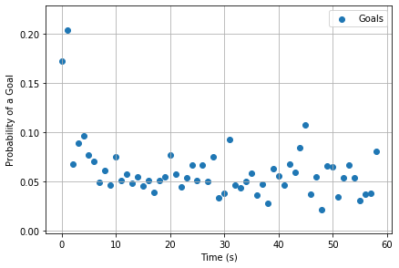
We can see that the probability of a goal is elevated when the shot occurs 0 or 1 s after the prior save, which is broadly in line with the previous NHL analysis. It is worth bearing in mind that getting the timing of shots correct must be very challenging when trying to record shots in real time, so there will be some inaccuracies in this data. In this dataset I’ll consider rebounds as shots that occur within 0 or 1 s after a save. This lead to 558 shots being classified as a rebound, out of 25263 total shots, equal to 2.2%. Sheffield and Dundee generated the highest number of rebounds with 121 and 72, respectively. Kevin Dufour (Dundee Stars) took the highest number of rebound shots with 15, while Liam Morgan (Belfast Giants) scored off the most rebounds - 4 in 8.
Looking at the probability of a shot attempt resulting in a goal, we have 5.4% of non-rebound shots are goals, but 17.9% of rebound shots are goals. 55.1% of non-rebound and 53.7% rebound shot attempts were saved, while only 9.8% of rebound shots were blocked and 18.6% went wide - down from 16.4% and 23.1% for non-rebound shots, presumably due to rebounds occuring closer to the goal
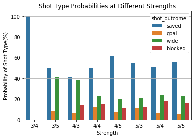
Another thing to take into account is whether there is a powerplay occurring or not. You would expect a team on a powerplay to have better control of the puck which may lead to higher quality shots and therefore a higher probability of a goal being scored from a particular distance. First, let’s take a look at all shots across different scenarios (powerplay, shorthanded, even strength). I’ve removed shots that occur in overtime from this data, overtime is played with each team icing 3 outskaters each. If a penalty occurs, or if a penalty runs over from regulation time, then the teams will play 4-on-3 until the penalty expires and then will play 4-on-4 until the next whistle when they revert to 3-on-3. It was not possible to get the required information to ascertain when teams were playing 4-on-4 in overtime so I decided to omit these shots from this analysis, I have also excluded all empty net goals from this as well.
| Strength | Total Shot Attempts | Total Goals |
|---|---|---|
| 3/4 | 2 | 0 |
| 3/5 | 12 | 1 |
| 4/3 | 29 | 2 |
| 4/4 | 252 | 29 |
| 4/5 | 698 | 42 |
| 5/3 | 273 | 31 |
| 5/4 | 4769 | 325 |
| 5/5 | 18906 | 986 |
We can see that the probability of a shot resulting in a goal while 5-on-5 (5.2%) is lower than when a team has a 5-on-4 (6.8%) or a 5-on-3 (11.4%) powerplay. We also see that the probability of a shot resulting in a goal when a team is shorthanded is also higher (6.0% when on a 4-on-5 penalty kill), also note that the probability of a goal while 4-on-4 is also a lot higher at 11.5%.
As mentioned earlier, the times of shots definitely have some inaccuracies, and therefore these numbers may be inaccurate. The number of goals at each strength is correct as these were taken from the gamesheets which should be accurate, but the other shots may not be accurate.
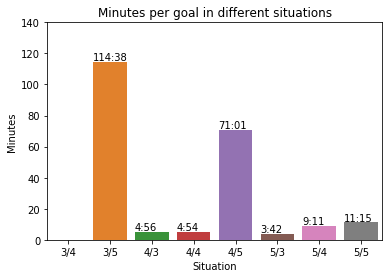
From the penalty data I can also calculate the time per goal at each different strength. We can see that there is a goal every 3:42 of 5-on-3 time, so teams need almost two full 5-on-3 powerplays to score a goal (a minor penalty lasts for 2 minutes). Teams require almost five full 5-on-4 penalties to score a goal - 9:11 per goal - which matches with most team’s powerplay which ranged from 15.0% (Glasgow Clan) to 27.8% (Cardiff Devils). Interestingly, you’re more likely to score when 4-on-4 than any other situation - 5-on-3 aside - perhaps having more space on the ice leads to more goals. The time per goal when 4-on-3 is also very low, however there were only 2 goals scored in this case.
Now we can combine these two last pieces of information to look at the probability of a shot resulting in a goal under different situations. For all shots (rebounds and non-rebounds) 5.3%, 6.1%, and 7.1% resulted in goals when even strength, shorthanded, and on the powerplay, respectively. There was a slight decrease for non-rebound shots: 5.1% (even), 5.9% (SH), and 6.5% (PP), while for rebound shots the values were 14.7% (even), 10.5% (SH), and 27.5% (PP) - bearing in mind there were only 2 rebound goals scored while shorthanded.
Let’s take a look at the probability of a shot resulting in a goal as a function of distance when on a powerplay or even strength, and whether a shot is a rebound or not. The number of shots is quite low when compared to the NHL, where there are 31 teams playing 82 games per season, so we may expect some noise in the plots.
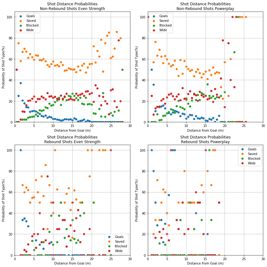
The noise is particularly noticeable for rebound shots (only 2.2% of all shots) and on the powerplay, short handed shots have been omitted due to their low numbers. One interesting finding here is the shape of the blocked shots curves for non-rebound shots. When even strength the probability of a shot being blocked peaks at a distance approximately 15 m from the goal before reducing, however the same phenomena is not present on the powerplay where it appears the probability of a blocked shot plateaus after 15 m.
We’re mainly interested in goals, so let’s compare the probability of a shot attempt resulting in a goal under these 4 situations.
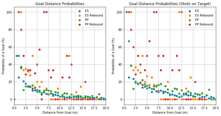
The left plot shows the probabiltiy of a shot attempt resulting in a goal as a function of situation, shot type, and distance from the net. The right hand plot shows the same, however the normalisation is performed to total shots on target (saves + goals) - this is what is typically referred to as a shot in hockey. The x limit has been reduced to 20 m as the probabilities were very low outside of this range. The rebound data is very noisy due to the low number of shots and goals, however we can see an elevated probability of a goal when on the powerplay for non-rebound shots, particularly in the range 7.5 m - 12.5 m from the goal.
Shot Angle
The final feature we’ll take a look at is shot angle - one would expect shots from tight angles to be more difficult to score due to the reduced solid angle of the goal, while shots from in front of the goal have a larger solid angle to aim for. On the other hand, netminders often try to push rebounds out to the sides and rebounds have a higher probability of resulting in a goal. First let’s take a look at the angular distribution of shots and goals, we’ll define a shot that is taken directly parallel to the centre of the goal to have an angle of 0 degrees, a shot from the right wing to have an angle < 0 degrees, and a shot from the left wing to have an angle of > 0 degrees. Therefore a shot from the goal line on the right wing has an angle of -90 degrees, and a shot from the goal line on the left wing has an angle of 90 degrees.
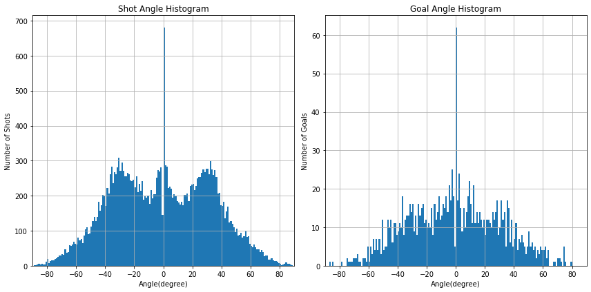
The histograms above are binned at 1 degree intervals, and the plots show a few interesting features. Firstly, shots occur from either directly in front of the net (an angle of close to 0) or at an angle of +/- 30 degrees from the net. The angular range of 20 to 40 degrees includes the area inline with the face off circles just inside the blueline - i.e. where a defenceman would normally be positioned, so this explains the spike here. The spike around 0 degrees can be seen from the shot heat maps earlier on, which all showed a hot spot around the front of the net for shots. There is a very high peak in the range -0.5 to 0.5 degree which appears to be an outlier. These shots were recorded with an x position of exactly 0, i.e. directly in line with the centre of the goal, which may suggest there was some error with recording the data? I am not sure.
We can also take a look at the probability of each shot type as a function of shot angle, which has been shown below. The goals have also been plotted separately as they were difficult to see in the original plot. The goals have been separated into left wing and right wing.
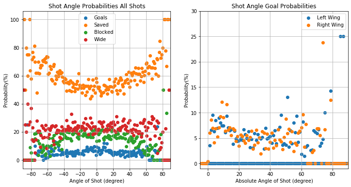
Here we can see the probability of a shot being saved appears to be lower when a shot is taken from straight in front of the net (angle close to 0 degrees) and the probability of a goal increases in this range. We can also see that the probability of a shot being blocked increases at lower absolute angles (i.e. close to 0 degrees), while the probability of a shot going wide does not appear to vary too much with angle. Visual inspection of the data suggests that shooting from the left or right wing does not appear to change these probabilities too much.
Building a Shot Model using Logistic Regression
The shot data analysis suggests that the probability that a shot attempt results in a goal is dependant on the strength (powerplay, even, or shorthanded), the distance and angle that the shot is taken from, and whether the shot is a rebound. We can use these features to build a model to predict whether a shot attempt will result in a goal, with the caveat that there are data quality issues that may reduce the performance of any model - possible inaccuracy in shot positioning, inaccuracy in the timing of the shot leading to incorrect estimates of whether a shot is a rebound or how many players were on the ice at the time of the shot.
I treated the problem as a binary classification problem - a shot attempt is either a goal or not, it doesn’t matter whether the shot missed, blocked, or was saved these cases were labelled as no goal - and solved it by implementing a Logistic Regression Classifier in Scikit-Learn. I used four features for the model, 2 numeric and 2 categorical:
- Adjusted Shot Distance: Previous analysis has suggested that recorded shot distance varies by which arena hosted the game (in the NHL). To account for this the mean shot distance in each arena is calculated and the adjusted shot distance is the difference between the shot distance and the mean.
- Absolute Shot Angle: From the analysis above it appears that the probability of a goal is dependant on the angle at which a shot was taken but not whether that shot was from the left or right wing. Therefore the absolute vaule of the angle was used
- Situation: The situations were combined to powerplay, even strength, and shorthanded, rather than specifying 5-on-4, 5-on-3 etc. This was because some situations occurred very rarely and I didn’t want any extreme cases to skew the results.
- Rebound: As described in the analysis, a shot was classified as a rebound if it occurred 0 or 1 seconds after a save.
The numeric variables (angle and distance) were converted to z-scores prior to fitting the model, which was implemented using Scikit-learn and the logistic regression optimisation was solved with L2 regularisation applied (it’s applied by default in scikit-learn). I evaluated the model using a repeated stratified K-fold cross validation (10 splits, 3 repetitions) technique and calculated the mean AUC of the ROC curve across the folds. Let’s first define what this means:
- Training & test set: We separate out the dataset into a training and test set, we fit the logistic regression model using the training set and evaluate the performance on the test set.
- K-fold Cross Validation: We take the whole dataset and split into $k$ equally sized subsets, each subset is treated as the test set in turn, the rest of the subsets are treated as the training set and used to fit the model. We end up with $k$ models and therefore $k$ values of the evaluation metric (AUC of the ROC curve in this case). I used $k = 10$ so $10$% of the dataset was used as the test set in each iteration of the cross validation.
- Stratified Cross Validation: This is the same as the above, except that the ratio of the classes (goal or no goal) is kept the same in each of the subsets. This is important when having many more instances of one class than the other. In our cases there are many more no goals than goals.
- Repeated Stratified Cross Validation: We repeat the stratified cross validation $n$ times with randomisation to ensure we do not just repeat the same splits. I used $n = 3$.
- ROC Curve: The receiver operating characteristic (ROC) curve is a plot that shows the diagnostic ability of a binary classifier. By varying the discrimination threshold of the classified (i.e. we say a shot is classified as a goal in the model when $P(G) > t$ for some threshold $0 \leq t \leq 1$) we get a different number of false positives (no goals classified as goals) and true positives (goals correctly classified). The ROC curve is a plot of the true positive rate against the false positive rate. For example, if we set $t = 0$ then all shots will be predicted to result in a goal and we therefore have a $100$% true positive rate but also a $100$% false positive rate. Conversely, if we set $t= 1$ then all shots will be classified as no goal and we will have a $0$% false positive rate but also a $0$% true positive rate.
- AUC of the ROC Curve: We integrate the ROC curve to calculate the AUC - the higher the AUC the better the model. An AUC $= 1$ would be the perfect model. If we have an AUC $=0.5$ then the model is not able to correctly differentiate between goals and non goals. We can think of the AUC as the probability the model will be able to distinguish between the goal and non-goal classes.
Previous analysis of shot data from the NHL has resulted in an AUC of $0.729$ (this appears to be without any cross validation) when using adjusted distance, rebound, situation, angle, shot after a give away, and shot type (e.g. wrap, slap, etc). They also reported a Kolmogorov-Smirnov (KS) statistic of 36.67. The KS statistic is calculated by applying the model to the test set, ordering the values of $P(G)$ and splitting into 10 equally sized subsets. The cumulative distribution of the true goals and non-goals is calculated, and the maximum difference between these two values is the KS statistic, which ranges from 0 to 100 (the larger the better).
After applying the cross-validation the mean value of the ROC AUC was $0.74 +/- 0.05$ at the 95% confidence level. This is well matched with the previous NHL analysis and a more modern NHL analysis that uses more features, which is promising. The KS statistic was $37 +/- 7$, which is again well matched to the previous analyses, however the variation in this statistic is quite high.
Applying the model to the entire dataset allows us to calculate the training set allows us to calculate the coefficients of the model and look at the importance of each feature. Each coefficient in the model is the expected change in the log odds of scoring a goal for a unit increase in the corresponding predictor variable, holding the other predictor variables constant. . The coefficients of the model have been plotted below.
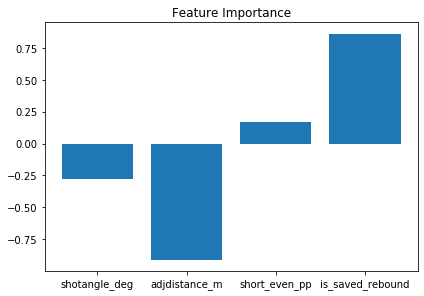
The interpretation of the coefficients is slightly complicated by the normalisation I performed (converting to z-scores), but lets take a look at these values. for each unit increase in normalised shot angle, keeping the other variables constant, leads to a reduction in the odds of a goal by 25%. This suggests a higher shooting angle, i.e. a shot from a tighter angle, the lower the probability of a goal. The adjusted shot distance has an even higher effect on the odds of the goal, each unit increase in the normalised adjusted shot distance decreases the odds of a goal by 60%, while if a goal is rebound we see an increase in the odds by 136%. Fortunately, this matches with the general trends we saw in the data analysis.
Building a Shot Model using a Random Forest
I also tried building a model using a Random Forest classifier. A Random Forest is an ensemble learning method, that generates a number of decision trees by sampling, with replacement, a subset of the training data to construct each tree. The probability of a data point from the test set belonging to a particular class (e.g. a goal) is the number of decision trees that predict that data point to be a goal divided by the total number of decision trees constructed.
Random Forests have a number of hyperparameters that require optimisation, I used a randomised search cross-validation method on the following parameters:
n_estimators: The number of trees in the forest.max_features: The number of features to consider when looking for the best split.max_depth: The maximum depth of the trees.min_samples_split: The minimum number of samples required to split an internal node.min_samples_leaf: The minimum number of samples required to be at a leaf node.
To optimise some the hyperparameters I used a randomised search technique with 5-fold cross-validation using the RandomizedSearchCV method in scikit-learn.
After applying the cross-validation the mean value of the ROC AUC was $0.73 +/- 0.05$ at the 95% confidence level. The KS statistic was $36 +/- 7$. Both of these values match the logistic regression model.
We can directly extract the feature importance from the model in scikit-learn, which will tell us how important each feature is to the prediction. A random forest is made up of a number of decision trees, every node in the decisions trees splits the dataset into 2 subsets on a single feature, designed in such a way that the data points with the same labels (goal or no goal) end up in the same subset. How to split is based on the Gini impurity, which is a measure of how often a randomly chosen element from the set would be incorrectly labelled if it was randomly labelled according to the distribution of labels in the subset. To calculate it we use $$G = \sum_{i=1}^{C} p(i)(1-p(i)),$$ where $C$ is the number of classes ($2$ in our case) and $p(i)$ is the probability of picking a datapoint with class $i$. In the perfect split, where all elements are correctly labelled, the Gini impurity is 0. For our entire dataset we have $1489$ goals and $23525$ no goals - let’s say we didn’t split the dataset at all, then p(goal) = 0.06, p(nogoal) = 0.94 and $$G = 0.06x0.94 + 0.06x0.94 = 0.11.$$ To train a decision tree, we find the split that minimises the Gini impurity. After training a Random Forest we can calculate the mean decrease in the Gini impurity across the decision trees that make up the Forest. For our model we had the following feature importance values
| Feature | Importance |
|---|---|
| Shot Angle | 0.30 |
| Adjusted Distance | 0.62 |
| Situation | 0.03 |
| Rebound | 0.05 |
which shows that the adjusted distance is the most important feature, followed by angle, situation, and rebound.
Calculating Shot Quality
Now we have our trained models, we can calculate a few more metrics for the teams. For example, we can calculate the probability of a goal from anywhere on the ice and the quality of each shot taken - that is the probability of each shot resulting in a goal. First, lets generate a grid of points in the offensive zone, set the situation to be Even Strength, and each shot to not be a rebound. We can then calculate the probability that a shot from each point on the ice results in a goal. We can then repeat this for power play and shorthanded situations, and also for rebounds. The images below show the modelled goal probability in these situations.
Firstly, let’s look at the Logistic Regression model. I’ve included the contour lines for ease of interpretation.
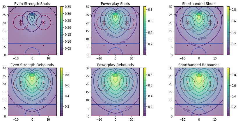
The first thing to notice is that some of the probability values are very high, particularly close in to the goal and on the rebound. Some of this may be due to a lack of data in certain situations, for example short handed rebounds. These high probability values are concerning to me.
Now let’s take a look at the Random Forest model. I’ve kept the colour scale the same as the previous example to compare, however I remove the contour lines as it was difficult to read the numbers.
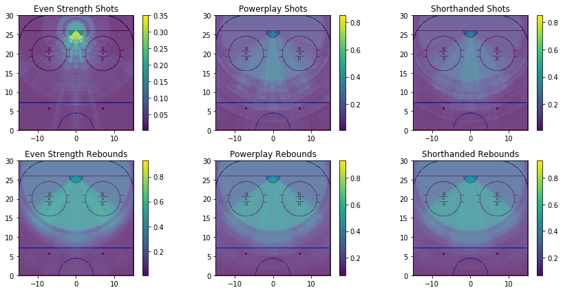
The first thing is to notice is that, due to the structure of the Random Forest, we now have step changes in the probability of a shot resulting in a goal. The probabilities are also lower than those calculated by the logistic regression model when the shot is close to the goal. We can also see that when even handed and the shot is not a rebound the probability of a shot attempt resulting in a goal is very low, only increasing close to the net. There is also a zone between the faceoff circles with a slightly elevated probability of scoring. On the powerplay the probability of a goal is increased, particularly further away from the goal than when even strength, and similar is seen when shorthanded. When a shot is classified as a rebound, we can see a much higher probability of scoring - note the increased range on the colour bar - and in particular a higher chance of scoring at a higher angle. This is an interesting feature and could be something to look at in more detail in the future.
The final thing I have done with the models is to calculate the average shot quality for and against each team. To calculate these values I sum up the probability of each shot resulting in a goal for/against each team, this gives the expected number of goals for/against each team. I normalise this per game - because the season finished early teams had played a different number of games - then multiply this by the league-wide average shots per game and divide by the team shots per game. This accounts for teams taking/conceding more or less shots per game than the average. I then divide these values by the league wide average goals per game to give me a normalised shot quality for/against per team.
The models give me the probability for each regular shot being a goal, I set the probability of a penalty shot being scored as 2/19 as there were 2 PS goals in 19 attempts. Then I set probability of an ENG shot being scored as 1 as I had no other data. Finally, I removed all over time shots from the dataframe and only focussed on regulation time shots and goals. I then used all of these values to calculate the shot quality for (SQF) and against (SQA) for each team, which should independent of the number shots taken and of goaltending.
First let’s look at the SQA for each team, calculated using the two models.
| Team | LogReg | RF |
|---|---|---|
| Belfast Giants | 1.02 | 1.02 |
| Cardiff Devils | 0.99 | 1.00 |
| Coventry Blaze | 1.00 | 0.99 |
| Dundee Stars | 0.98 | 0.96 |
| Fife Flyers | 1.07 | 1.06 |
| Glasgow Clan | 0.97 | 0.96 |
| Guildford Flames | 0.92 | 0.91 |
| Manchester Storm | 1.06 | 1.05 |
| Nottingham Panthers | 1.01 | 0.99 |
| Sheffield Steelers | 0.99 | 0.98 |
To interpret this, a team with SQA $ = 1.05$ would concede $5$% more goals than a team with an SQA of $1$, all other things kept constant. We can see that Manchester & Fife, two of the bottom three sides in the league had a higher SQA than the other sides. On the other end, Guildford had the lowest SQA. What is interesting is that Dundee and Glasgow, two lower ranking teams also had lower SQA than teams at the top of the table.
The SQF values are given below for the two models.
| Team | LogReg | RF |
|---|---|---|
| Belfast Giants | 1.05 | 1.02 |
| Cardiff Devils | 1.01 | 1.01 |
| Coventry Blaze | 1.03 | 1.02 |
| Dundee Stars | 1.08 | 1.05 |
| Fife Flyers | 0.96 | 0.97 |
| Glasgow Clan | 1.03 | 1.04 |
| Guildford Flames | 0.95 | 0.94 |
| Manchester Storm | 0.88 | 0.85 |
| Nottingham Panthers | 0.98 | 0.98 |
| Sheffield Steelers | 1.04 | 1.04 |
Manchester are the obvious outliers here, and they struggled to score last season. Guildford and Fife also have a low SQF. Again, Dundee and Glasgow’s values do not reflect their standing in the league.
Summary
I scraped the EIHL shot data to analyse where teams have shots and built 2 models to predict whether a shot attempt would result in a goal or not. This project initially started out as just scraping the data and looking at where teams took shots from and where they scored from, however it soon became something much bigger! The values of the metrics used to evaluate the model match well with previous NHL analysis, which is encouraging, however there are likely to be inaccuracies in the model due to data quality issues. To improve the model, beyond increasing the quality of the data, would require recording extra information about the events on the ice as they do for the NHL. On the data quality side, there were some issues with the recorded time of the shots and it would be useful to record how many skaters were on the ice when each shot was taken, rather than try to calculate this from the penalty data. Overall, I am happy with the models outcome given the data issues.
I used Logistic Regression and a Random Forest for the models, but there were other options. One paper I saw also used XGBoost, which I may also try at a later date. I may also look at considering only shots on target - either saves or goals - which tell me more about the performance of the netminders rather than the whole defensive unit of each team. One downside of this is that the number of data points becomes reduced.
Getting the data & Scripts
I have made the Python notebooks available on my github here. I have not included the raw shot or gamesheet data, however I have included the code to scrape it - note that it will take some time as I included a pause to reduce the number of calls to the EIHL websites per second.
References
Elite League Website: www.eliteleague.co.uk
The Scott method of Bandwidth estimation: D.W. Scott, “Multivariate Density Estimation: Theory, Practice, and Visualization”, John Wiley & Sons, New York, Chicester, 1992.
A New Expected Goal Model for Predicting Goals in the NHL, EvolvingWild
Scikit-learn: Machine Learning in Python, Pedregosa et al., JMLR 12, pp. 2825-2830, 2011.